
ML predictions on Breast Cancer
Walkabout of ML using Caret
This post is going to describe a step-by-step ML analysis using Caret to build a classification model based on logistic regression. Logistic regression is a supervised learning method that predicts class membership and it is characterised for the S-shaped curve of the logistic function. For further reading on logistic regression see.
The dataset I am going to work with has features on breast cancer digitized images of nuclei collected with fine needle aspirate (FNA) from a breast mass. This data is a Kaggle competition to predict whether the cancer is benign or malignant. For each cell nucleus ten features are computed and for each feature there is information on mean, standard error and the "worst’/largest (mean of the three largest values) of each features. So in total there are 30 features. And there is information about two attributes: diagnosis (benign or malignant) and patient ID number.
library(tidyverse)
library(RCurl) #to read data
library(caret) #to do ML
library(caretEnsemble) #to make ensembles of caret models
library(GGally) #to get high-level visualizations
library(DMwR) # to balance the unbalanced class
library(FSelector) #to remove unnecessary features
Basically a ML workflow follows these steps:
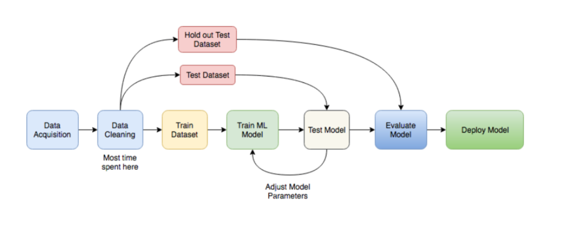
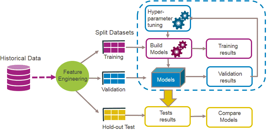
ML
So lets follow those steps to build a classifier model that predicts breast cancer diagnosis!
Data acquisition
x <- getURL("https://raw.githubusercontent.com/demar01/blog/master/static/blog/%202020-09-02/data-1.csv")
breast.cancer.raw<- read.csv(text = x)
Data cleaning
breast.cancer.raw<-breast.cancer.raw[,-33]
cat("The dimension of data set is (", dim(breast.cancer.raw), ")")
## The dimension of data set is ( 569 32 )bcancer <- breast.cancer.raw %>%
dplyr::select(-id)
bcancer$diagnosis <- as.factor(bcancer$diagnosis)
names(bcancer)[9]<-"concave.points_mean"
names(bcancer)[19]<-"concave.points_se"
names(bcancer)[29]<-"concave.points_worst"
bcancer %>%
count(diagnosis)## diagnosis n
## 1 B 357
## 2 M 212Feature Engineering
Feature engineering allows to capture the important, interesting features in the dataset with respect to an outcome variable (aka diagnosis).
There are multiple ways to assess feature importance.
We can use the random forest method to find the weights of attributes using random.forest.importance function and cutoff.k to select a subset from a ranked attributes.
attribute.scores <- random.forest.importance(diagnosis ~ ., bcancer)
Top_features<-cutoff.k(attribute.scores, k = 9) # Top 9 features

bcancer<-bcancer%>%
  dplyr::select(diagnosis,all_of(Top_features))
factor_variable_position<-c(1)
bcancer<-bcancer%>% mutate_at(.,vars(factor_variable_position),~as.factor(.))## Note: Using an external vector in selections is ambiguous.
## ℹ Use `all_of(factor_variable_position)` instead of `factor_variable_position` to silence this message.
## ℹ See <https://tidyselect.r-lib.org/reference/faq-external-vector.html>.
## This message is displayed once per session.We can have a look at the data globally:
bcancer %>%
ggpairs(mapping = aes(color = diagnosis))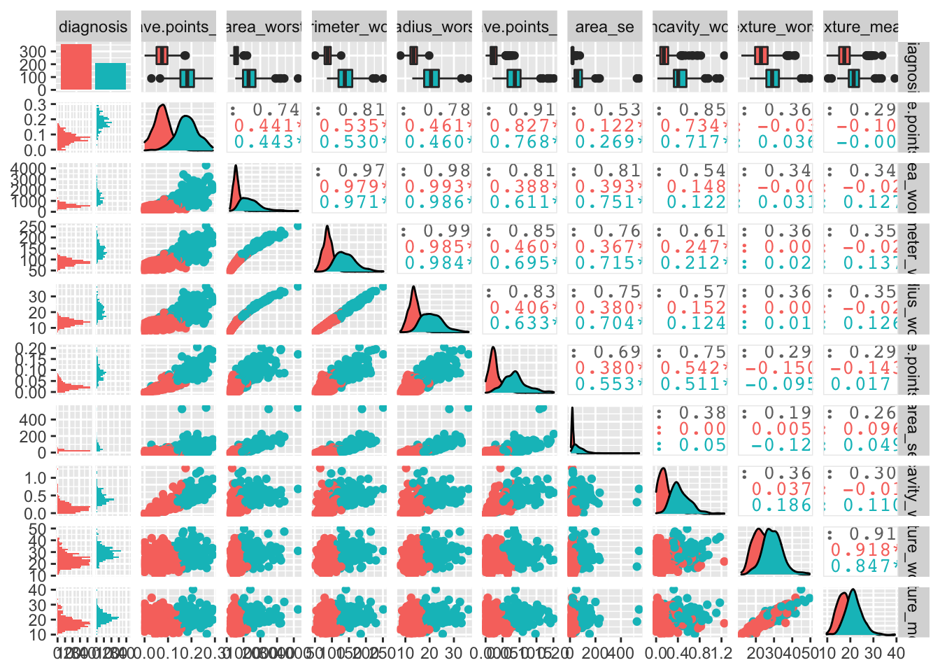
Spliting the data
partition <- createDataPartition(bcancer$diagnosis, p = 0.8, list = FALSE)
bcancerTrain<- bcancer[partition, ]
bcancerTest <- bcancer[-partition, ]
Scaling and standardising data
Scaling (divide by standard deviation) and standardising (mean substract) will help to reduce variance between features.
preProcess_scale_model <- preProcess(bcancerTrain, method = c("center", "scale"))
bcancerTrain <- predict(preProcess_scale_model, bcancerTrain)
bcancerTest <- predict(preProcess_scale_model, bcancerTest)
We can visualise how the features influence diagnosis:
featurePlot(x = bcancerTrain[, -1],
            y = bcancerTrain$diagnosis,
            plot = "density", main= "Density of predictive Features",
            strip=strip.custom(par.strip.text=list(cex=1)),
            scales = list(x = list(relation="free"),
                          y = list(relation="free")))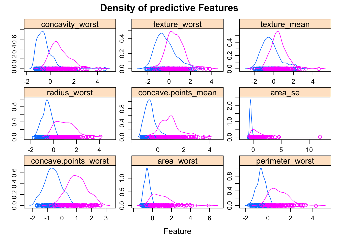
Features with a high predictive value have very different density curves for the outcome, both in terms of the height (kurtosis) and placement (skewness).
But, how are these variables correlated between each other? Ideally, not too much so they add additional information.
numericVarName <- names(which(sapply(bcancer, is.numeric)))
corr <- cor(bcancer[,numericVarName], use = 'pairwise.complete.obs')
ggcorrplot(corr, lab = TRUE, title = "Multicollinearity of predictive features")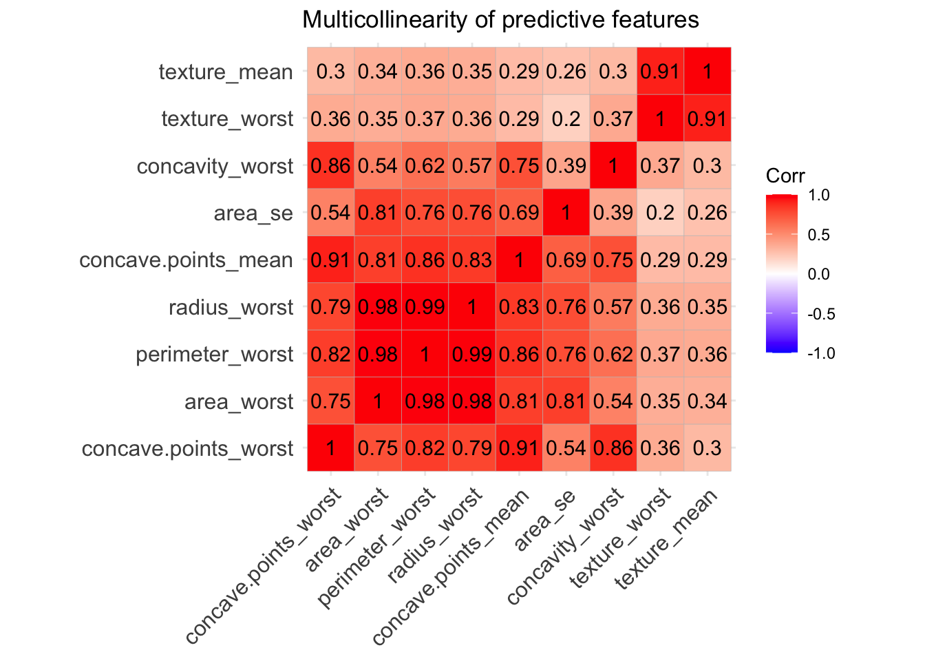 We can see that some of the variables - like area, radius and perdimeter- are highly correlated, which makes sense they are values that multiply the radius with a constant. So looking at the multicollinearity plot together with the feature plot for predictor variables we could make a guess of the important features that will be finally included in our predictive model.
From looking at those one could tell that area_se, texture_worst, concave.points_mean,concave.points_worst, area_worst.
We can see that some of the variables - like area, radius and perdimeter- are highly correlated, which makes sense they are values that multiply the radius with a constant. So looking at the multicollinearity plot together with the feature plot for predictor variables we could make a guess of the important features that will be finally included in our predictive model.
From looking at those one could tell that area_se, texture_worst, concave.points_mean,concave.points_worst, area_worst.
We could use Recursive Feature Elimination (RFE) to automatically select those important features to be finally included in our predictive model.
control <- rfeControl(functions = rfFuncs,
                      method = "repeatedcv",
                      number= 10,
                      repeats = 5,
                      verbose = FALSE,
                      allowParallel = TRUE)
outcomeName<-'diagnosis'
predictors<-names(bcancerTrain)[!names(bcancerTrain) %in% outcomeName]
bcancer_Pred_Profile <- rfe(bcancerTrain[,predictors], bcancerTrain[,outcomeName],
                         rfeControl = control)
print(bcancer_Pred_Profile)
The top 5 variables (out of 9): concave.points_worst, concave.points_mean, perimeter_worst, area_worst, radius_worst.
#Training data set
bcancerTrain <- bcancerTrain%>%
  select(diagnosis,concave.points_worst,
         texture_worst,
         area_se,
         area_worst,
         concave.points_mean)
#Test data set
bcancerTest <- bcancerTest%>%
  select(diagnosis,concave.points_worst,
         texture_worst,
         area_se,
         area_worst,
         concave.points_mean)
Dealing with class imbalance
Synthetic Minority Oversampling Technique (SMOTE) is used to re-balance an unbalanced classification, which is the case for this dataset.
bcancerTrain_smothe <- SMOTE(diagnosis~., data.frame(bcancerTrain),
                      perc.over = 100, perc.under = 200)
#Data after SMOTHE
round(prop.table(table(dplyr::select(bcancerTrain_smothe, diagnosis), exclude = NULL)),3)
##
## B M
## 0.5 0.5###Making multiple models and compare them individually
To train the model we initially have to specify the parameters used to create the model using the function trainControl. An important parameter is the resampling method used to predict the performance of the algorithm. We can use repeatedcv, which is a nested, k-fold repeated crossvalidation.
Then we can create a list of several train models with function caretList and train each model individually.
set.seed(2020)

trainControl <- trainControl(
  method="repeatedcv",
  number=10,                  #number of folds
  repeats=5,                  #number of repeats for each fold
  savePredictions="final",    #Saves predictions for tuning parameter
  classProbs=TRUE,
  allowParallel = TRUE        #allow parallel computing
  )
#Model List
algorithmList <- c("glmboost",'rpart',"rf","xgbTree","naive_bayes",
                   'earth', 'kknn',
                   "lda", "Linda","C5.0Tree","adaboost")
#Train models separately
models <- caretList(diagnosis~., data=bcancerTrain,
          trControl = trainControl, preProcess=c("center","scale"),
          methodList = algorithmList,metric = "Kappa")
## Loading required package: earth## Loading required package: Formula## Loading required package: plotmo## Loading required package: plotrix## Loading required package: TeachingDemos# Collect resamples and summary of models performances
results <- resamples(models)
bwplot(results)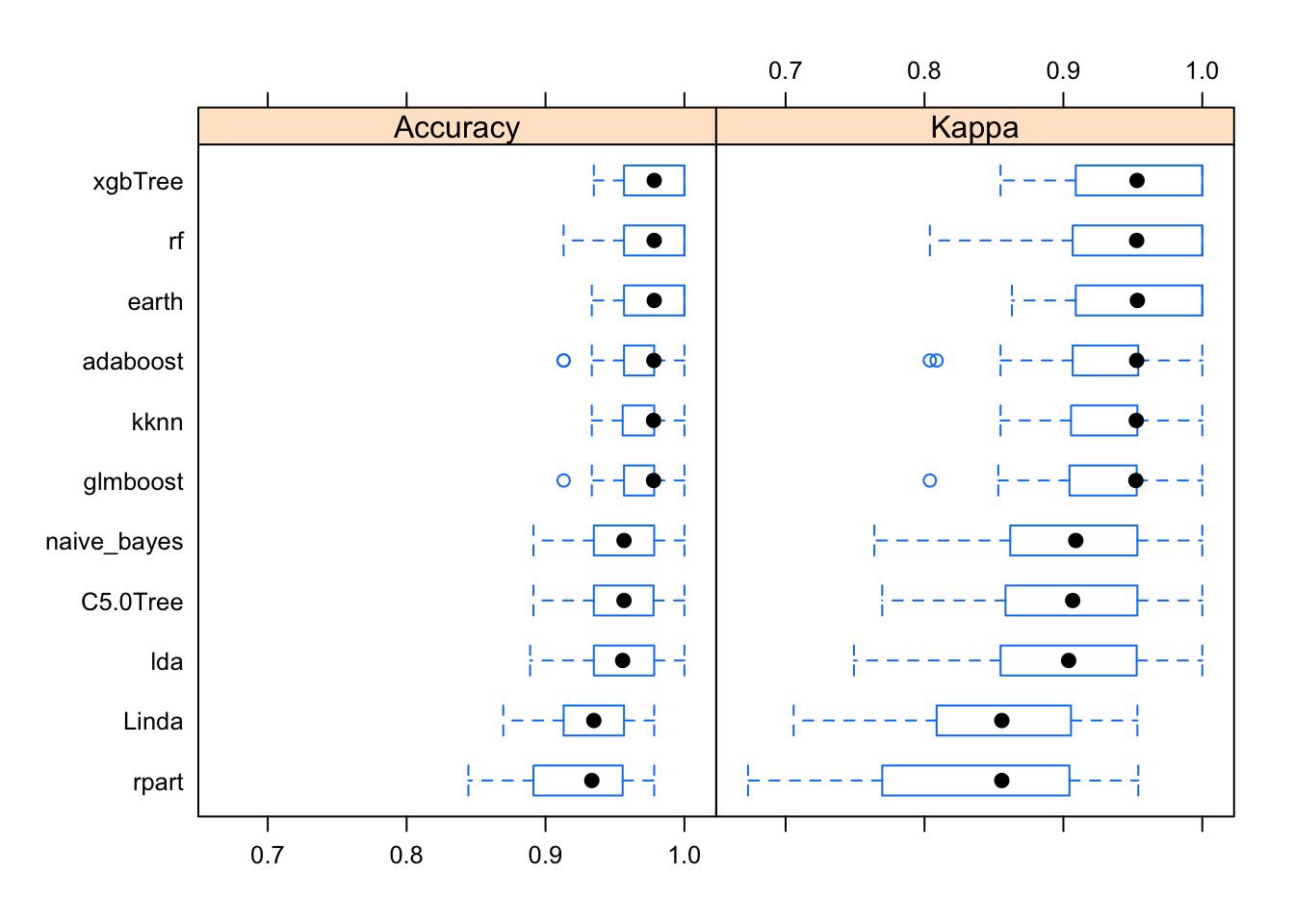
So, how do out models perform with the training data? Kappa (or Cohen’s Kappa) tell us how well the classifier performs compared to how well it would have performed simply by chance. So if Kappa=0 the agreement between breast cancer diagnostic decision prediction and reality is just by chance and if Kappa=1 the agreement is perfect. In our case, the best performing algorithm is xgbTree.
We could improve the model via hyperparameter tuning or by creating ensemble models. We can test the correlation between models, so if correlation is not high we could improve model performance by making ensembles of the model.
Modelcorr <- modelCor(results)
ggcorrplot(Modelcorr, lab = TRUE,title = "Correlation between model results")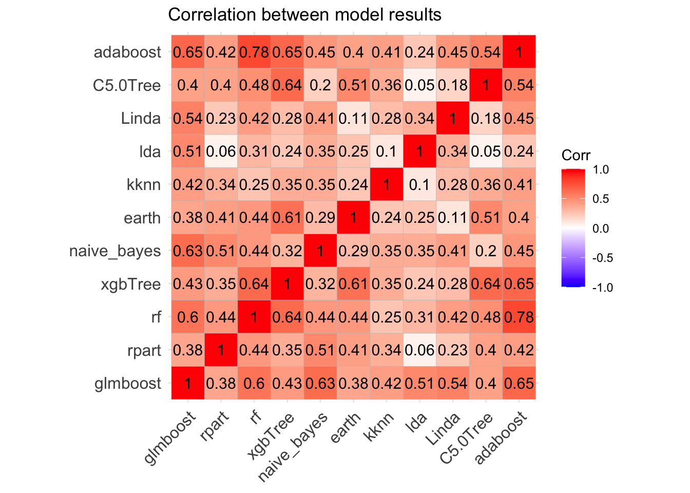
Great! Models correlation is not very high suggesting that each one may capture a different aspect of the data, and different models may perform best on different subsets of the data so one model may predict correctly cases where the other model predicts incorrectly. Therefore we could try to improve the overall performance combining the predictions of a number of models and making “meta-models” to ensemble collections of predictive models.
Adjust model by making ensembles of caret models
Similarly to before, we start specifying a new trainControl object and then we can use the caretStack function to create ensemble models from the list of caret models.
stackControl <- trainControl(method="repeatedcv",
                             number=10, repeats=5,
                             savePredictions=TRUE,
                             classProbs=TRUE,
                             allowParallel = TRUE
                             )
set.seed(2020)
stack.xgbTree <- caretStack(models, method="xgbTree",
                        metric="Kappa",trControl=stackControl)
Test Ensemble model with test dataset
stack_predicted_xgbTree<- predict(stack.xgbTree, newdata = bcancerTest)
head(stack_predicted_xgbTree, n = 10)
## [1] M M M M B M M M M M
## Levels: B MEvaluating the model
We can evaluate the model drawing a confusion matrix to analyzing the different types of errors of each ML model.
xgbTree.cmx <- caret::confusionMatrix(stack_predicted_xgbTree,
                                  bcancerTest$diagnosis, positive = "B")
draw_confusion_matrix(xgbTree.cmx)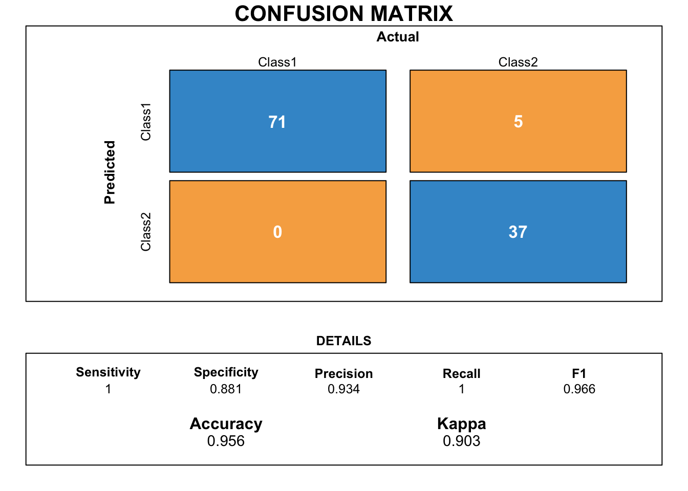
This confusion matrix shows the performance on prediction of the stack ensemble classification model when new/production data is passed through the model. The accuracy and Kappa show that this model is doing a pretty good job! Kappa for ensemble model is lower than that one for the base xgbTree, but bear in mind that the ensemble model had never seen the new testing data before!
Conclusions
We built stacked ensemble model gathered of individual based learners that has a pretty good probability of success when predicting breast cancer diagnosis.


