Motivation to do this exploration

A fantastic paper on the proteins that bind directly to the SARS-CoV-2 RNA in virally infected human cells has been recently published by Mathias Munschauer group The authors used purification and mass spectrometry (RAP-MS) to get the proteome that directly binds the SARS-CoV-2 when this infects human cells in an unbiased manner.

I got super curious on these data and wanted to explore myself. I wanted to visualised the protein-protein interaction (PPI) network of SARS-CoV-2 interacting proteins that helps understanding SARS-CoV-2 biology better.

library(here)
library(httr)
library(tidyverse)
library(data.table)
library(dplyr)
library(Matrix)
library(GGally)
library(network)
library(grid)

Building protein-protein interactions

PPI network can be built with STRING. We need String used Aliases anf the interaction values.

aliases <- fread("/Users/dermit01/Desktop/SCoV2-proteome-atlas-master/string_v11/9606.protein.aliases.v11.0.txt.gz", skip = 1, header = FALSE, col.names = c("STRINGid", "Alias", "source"))[,c(1,2)]

string_v11 <- fread("/Users/dermit01/Desktop/SCoV2-proteome-atlas-master/string_v11/9606.protein.links.v11.0.txt.gz")
gene2string <- (aliases$STRINGid)
names(gene2string) <- (aliases$Alias)

I obtained this function from the authors that is used to generated interaction database.

pull_string_v11 <- function(genes_keep, min_score = 0){
  
  string_genes_keep <- gene2string[genes_keep]
  string2gene <- names(string_genes_keep); names(string2gene) <- unname(string_genes_keep)
  #print(paste0("WARNING: ", paste(genes_keep[is.na(string2gene)], collapse = ","), " not found"))

    # Now filter
  data <- string_v11 %>% filter(combined_score > min_score) %>%
    filter(protein1 %in% unname(string_genes_keep) & protein2 %in% unname(string_genes_keep))
  
  data$node1 <- unname(string2gene[as.character(data$protein1)])
  data$node2 <- unname(string2gene[as.character(data$protein2)])
  data[complete.cases(data),c("node1", "node2", "combined_score")]
  
}

Once that we have the database we can visualise Covid19 interacting proteins

rap <- fread("https://raw.githubusercontent.com/demar01/blog/master/data/SCoV2/SCoV2_RAPms.txt") %>%
  filter(adj.P.Val.SCoV2.over.RMRP < 0.2 & species == "HOMO SAPIENS" & logFC.SCoV2.over.RMRP > 0)
rap_genes <- rap %>% pull(geneSymbol)

Initially the authors included edges between interacting proteins that have a combined interaction score of 550. I built a more restictive network with min_score 750

edges <- pull_string_v11(min_score = 750, genes_keep = rap_genes)

qc_genes <- c("SCFD1", "RAB6C", "RAB7A", "GDI2")

Building the network

levels = unique(c(edges$node1, edges$node2))
edges$node1 <- factor(edges$node1, levels = levels)
edges$node2 <- factor(edges$node2, levels = levels)

sm <- sparseMatrix(i = c(as.numeric(edges[["node1"]]), length(levels)), 
                   j = c(as.numeric(edges[["node2"]]), length(levels)), 
                   x  = c(edges[["combined_score"]], 0)) %>% data.matrix()
rownames(sm) <- levels
colnames(sm) <- levels

net <- network(sm)

Lets name the proteins for further colouring

# Show the full network
vesicle <- c("RAB7A","RAB6A","RAB1A","SCFD1","USO1", "GDI2")
viral_rna <- c("ATP1A1","CAPRIN1","CFL1","CSDE1","DDX1","DDX3X","EEF1A1","EEF2","EIF3E","EIF3G","EIF3L","EIF4B","EIF4G1","EIF4H","EIF5A","G3BP1","G3BP2",
               "HNRNPA1","HNRNPA2B1","IGF2BP1","IGF2BP2","LIN28B","LSM14A","MOV10","PABPC1","PCBP2","PEBP1","PFN1","PPIA","RPL13","RPL15","RPL18A","RPL21",
               "RPL28","RPL3","RPL36A","RPL6","RPL7A","RPL8","RPS11","RPS12","RPS14","RPS2","RPS26","RPS3","RPS4X","RPS5","SND1","SYNCRIP","UPF1","YBX1")

Lets get annotation for colouring

color_vec <- case_when(
  grepl("^RP", levels) ~ "RP",
  levels %in% viral_rna ~ "viral_rna_bind",
  TRUE ~ "Other"
)
table(color_vec)

net %v% "color" = color_vec

# Now do size
n_size_vec = rap$logFC.SCoV2.over.RMRP; names(n_size_vec) <- as.character(rap$geneSymbol)
size_vec <- unname(n_size_vec[levels])
net %v% "size_of_node" = size_vec

We can use the function ggnet2 for plotting network objects using ggplot2

set.seed(1)
pAI <- ggnet2(net, label = levels[color_vec != "Other"], color = "color",  legend.position = "right", mode = "fruchtermanreingold",
              layout.par = list(repulse.rad = 2000), alpha = 0.75, size = "size_of_node", size.cut = 10,
              palette = c("Other" = "grey", "RP" =  "dodgerblue4", "viral_rna_bind" = "purple2"),
              label.size = 2)  +  guides( size = FALSE)

#ggsave(here("static","img", "pAI.jpg"))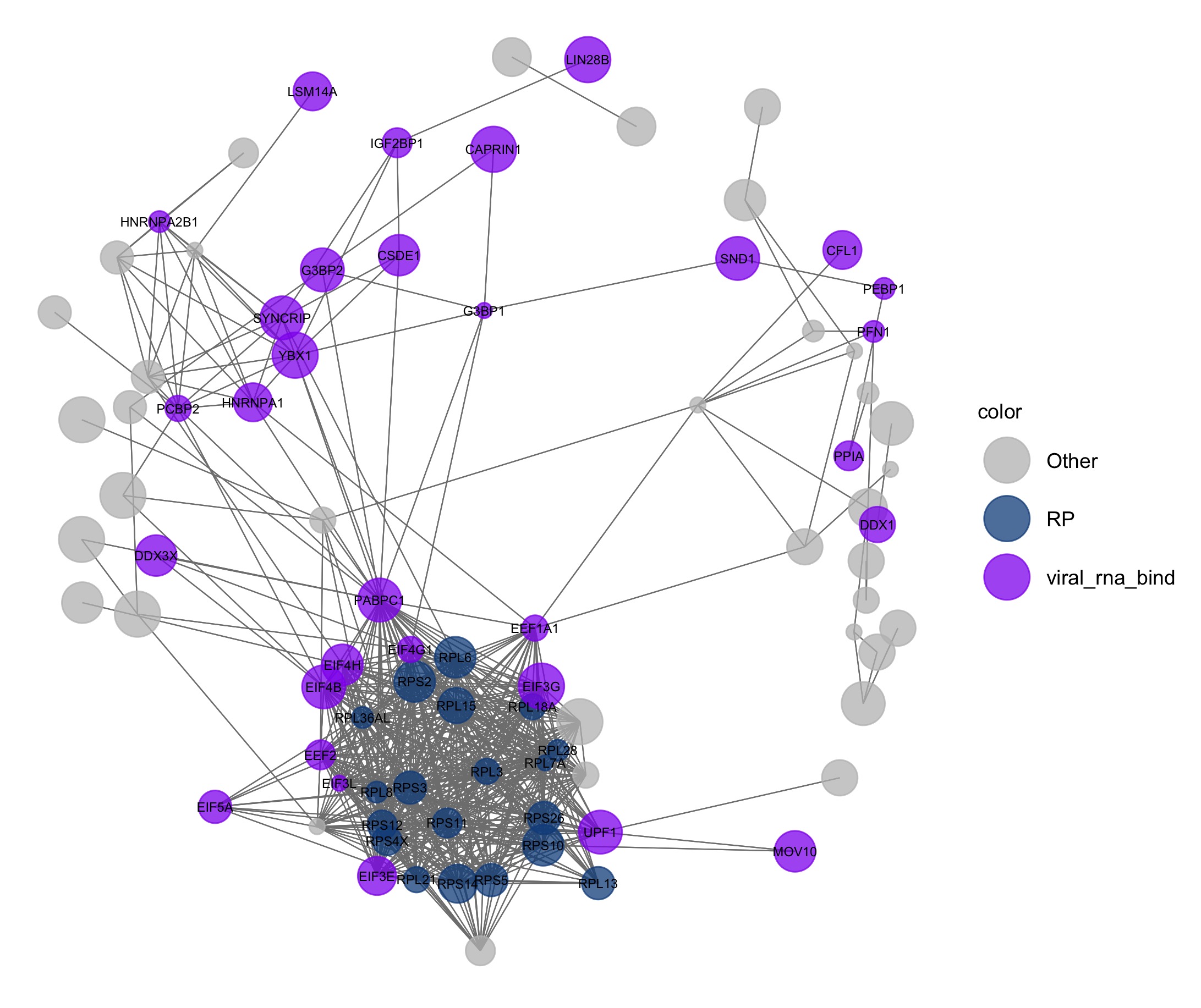

What of those proteins are druggable?

Reading the drug-target data

drugs <- fread("https://raw.githubusercontent.com/demar01/blog/e282080e210e6d7690402535025b5620046c7bb9/data/SCoV2/RAP-MS_dgidb_export_2020-06-29.tsv")

druggable <- drugs %>% pull(search_term) %>% unique()

net %v% "drug_target" = levels %in% druggable

set.seed(1)
pDrug <- ggnet2(net, label = druggable, color = "drug_target",  legend.position = "right", mode = "fruchtermanreingold",
              layout.par = list(repulse.rad = 2000), alpha = 0.75, size = "size_of_node", size.cut = 10,
              palette = c("FALSE" = "grey", "TRUE" = "firebrick"),
              label.size = 2) +  guides( size = FALSE)
pDrug

#ggsave(here("static","img", "pDrug.jpg"))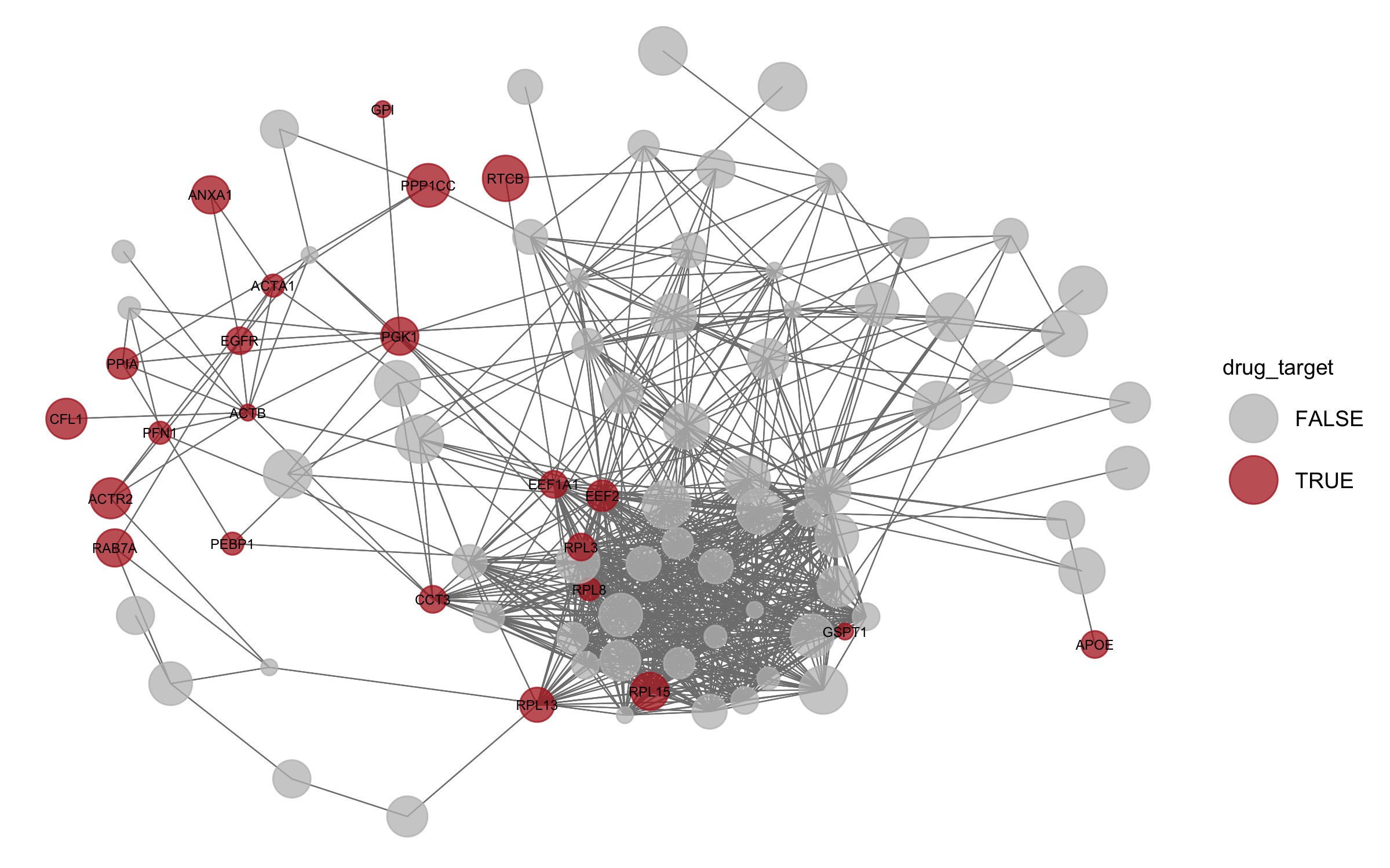

Conclusions

This is a fantastic resource of the direct SARS-CoV-2 RNA-protein interactome in infected human cells. obtained by RAP-MS. Very interestingly ANXA1 is a known target of dexamethasone, which according to newly emerging clinical trial data appears to show efficacy as a treatment for COVID-19.