XGBoost Phosphoproteome

Jul 1, 2020

Maria Dermit

6 minute read

library(dplyr)
library(ggplot2)
library(tidyverse)
library(tidymodels)
library(vip)
library(funscoR)

Motivation to do this comparison

Last year a great study on the funtional value of each phosphorylation site was published in Nature Biotechnology. In the paper, the authors gather phosphorylation sites from 6,801 proteomics experiments and created a reference phosphoproteome containing 119,809 human phosphosites. More importantly, the evaluated with a regression model the contribution of each phosphorylation site (funcitonal measured as a readout of anotation in PhosphoSitePlus. The aim of my analysis is to evaluate this using the tidymodels enviromennt.

Use useful functions withing this package to annotate a phosphorproteome

  annotated_phos <- annotate_sites(phosphoproteome)
  # annotate_sites is a function in the funscoR package that takes annotation files contained within the package to annotate a phosphoproteome with extra functional information
  Y_features <- preprocess_features(annotated_phos, "Y")
  # describe what this does

Phosphoproteome is an object where the authors gathered phosphorylation sites.

feat<-Y_features
goldreg <- psp
funclasses <- c("nonfunctional", "functional")
feat$is_regulatory <- funclasses[unclass(as.factor(row.names(feat) %in% paste(goldreg$acc, goldreg$position, sep = "_")))]
feat$is_regulatory <- as.factor(feat$is_regulatory)

For classification, I will use the is_regulatory variable.

EDA

feat<-feat %>% select(-residue)
feat$is_regulatory <- as.factor(feat$is_regulatory) 
feat<-feat %>% as_tibble()
feat %>% count(is_regulatory)

## # A tibble: 2 x 2
##   is_regulatory     n
##   <fct>         <int>
## 1 functional      400
## 2 nonfunctional  5879

Building the model

feat_split <- initial_split(feat, strata = is_regulatory)
feat_train <- training(feat_split)
feat_test <- testing(feat_split)

I split the data with the initial_split function of the rsample package

xgb_spec <- boost_tree(
  trees = 500, 
  tree_depth = tune(), min_n = tune(), 
  loss_reduction = tune(),                ## first three: model complexity
  sample_size = tune(), mtry = tune(),    ## randomness
  learn_rate = tune(),                    ## step size
) %>% 
  set_engine("xgboost") %>% 
  set_mode("classification")

This is going to build a model. I am going to use a classification model

xgb_grid <- grid_latin_hypercube(
  tree_depth(),
  min_n(),
  loss_reduction(),
  sample_size = sample_prop(),
  finalize(mtry(), feat_train),
  learn_rate(),
  size = 30 #increasing this number would lead to finner tree exploration
)

xgb_wf <- workflow() %>%
  add_formula(is_regulatory ~ .) %>%
  add_model(xgb_spec)

The specified model goes into a workflow

set.seed(123)

vb_folds <- vfold_cv(feat_train, strata = is_regulatory)

vb_folds

## #  10-fold cross-validation using stratification 
## # A tibble: 10 x 2
##    splits             id    
##    <list>             <chr> 
##  1 <split [4.2K/471]> Fold01
##  2 <split [4.2K/471]> Fold02
##  3 <split [4.2K/471]> Fold03
##  4 <split [4.2K/471]> Fold04
##  5 <split [4.2K/471]> Fold05
##  6 <split [4.2K/471]> Fold06
##  7 <split [4.2K/471]> Fold07
##  8 <split [4.2K/471]> Fold08
##  9 <split [4.2K/471]> Fold09
## 10 <split [4.2K/471]> Fold10

This creates cross-validation resamples (vfold_cv from the rsample package) to tune the model.

doParallel::registerDoParallel()
set.seed(234)
xgb_res <- tune_grid(
  xgb_wf,
  resamples = vb_folds,
  grid = xgb_grid,
  control = control_grid(save_pred = TRUE)
)

xgb_res

## #  10-fold cross-validation using stratification 
## # A tibble: 10 x 5
##    splits            id     .metrics         .notes         .predictions        
##    <list>            <chr>  <list>           <list>         <list>              
##  1 <split [4.2K/471… Fold01 <tibble [60 × 9… <tibble [0 × … <tibble [14,130 × 1…
##  2 <split [4.2K/471… Fold02 <tibble [60 × 9… <tibble [0 × … <tibble [14,130 × 1…
##  3 <split [4.2K/471… Fold03 <tibble [60 × 9… <tibble [0 × … <tibble [14,130 × 1…
##  4 <split [4.2K/471… Fold04 <tibble [60 × 9… <tibble [0 × … <tibble [14,130 × 1…
##  5 <split [4.2K/471… Fold05 <tibble [60 × 9… <tibble [0 × … <tibble [14,130 × 1…
##  6 <split [4.2K/471… Fold06 <tibble [60 × 9… <tibble [0 × … <tibble [14,130 × 1…
##  7 <split [4.2K/471… Fold07 <tibble [60 × 9… <tibble [0 × … <tibble [14,130 × 1…
##  8 <split [4.2K/471… Fold08 <tibble [60 × 9… <tibble [0 × … <tibble [14,130 × 1…
##  9 <split [4.2K/471… Fold09 <tibble [60 × 9… <tibble [0 × … <tibble [14,130 × 1…
## 10 <split [4.2K/471… Fold10 <tibble [60 × 9… <tibble [0 × … <tibble [14,130 × 1…

This takes a long time, but doing parallel speeds up the process

collect_metrics(xgb_res)

## # A tibble: 60 x 11
##     mtry min_n tree_depth learn_rate loss_reduction sample_size .metric
##    <int> <int>      <int>      <dbl>          <dbl>       <dbl> <chr>  
##  1     2    23          8   1.03e- 4   0.000363           0.404 accura…
##  2     2    23          8   1.03e- 4   0.000363           0.404 roc_auc
##  3     3     5          5   5.62e- 6   0.0125             0.923 accura…
##  4     3     5          5   5.62e- 6   0.0125             0.923 roc_auc
##  5     4    17         13   7.53e- 5   0.0000000245       0.516 accura…
##  6     4    17         13   7.53e- 5   0.0000000245       0.516 roc_auc
##  7     5    28          7   4.96e- 8  13.0                0.440 accura…
##  8     5    28          7   4.96e- 8  13.0                0.440 roc_auc
##  9     6    13         13   1.25e-10   0.000200           0.975 accura…
## 10     6    13         13   1.25e-10   0.000200           0.975 roc_auc
## # … with 50 more rows, and 4 more variables: .estimator <chr>, mean <dbl>,
## #   n <int>, std_err <dbl>

The results of tune_grid can be explored with this function of the tune package

Using visualization to understand results

xgb_res %>%
  collect_metrics() %>%
  filter(.metric == "roc_auc") %>%
  select(mean, mtry:sample_size) %>%
  pivot_longer(mtry:sample_size,
               values_to = "value",
               names_to = "parameter"
  ) %>%
  ggplot(aes(value, mean, color = parameter)) +
  geom_point(alpha = 0.8, show.legend = FALSE) +
  facet_wrap(~parameter, scales = "free_x") +
  labs(x = NULL, y = "AUC")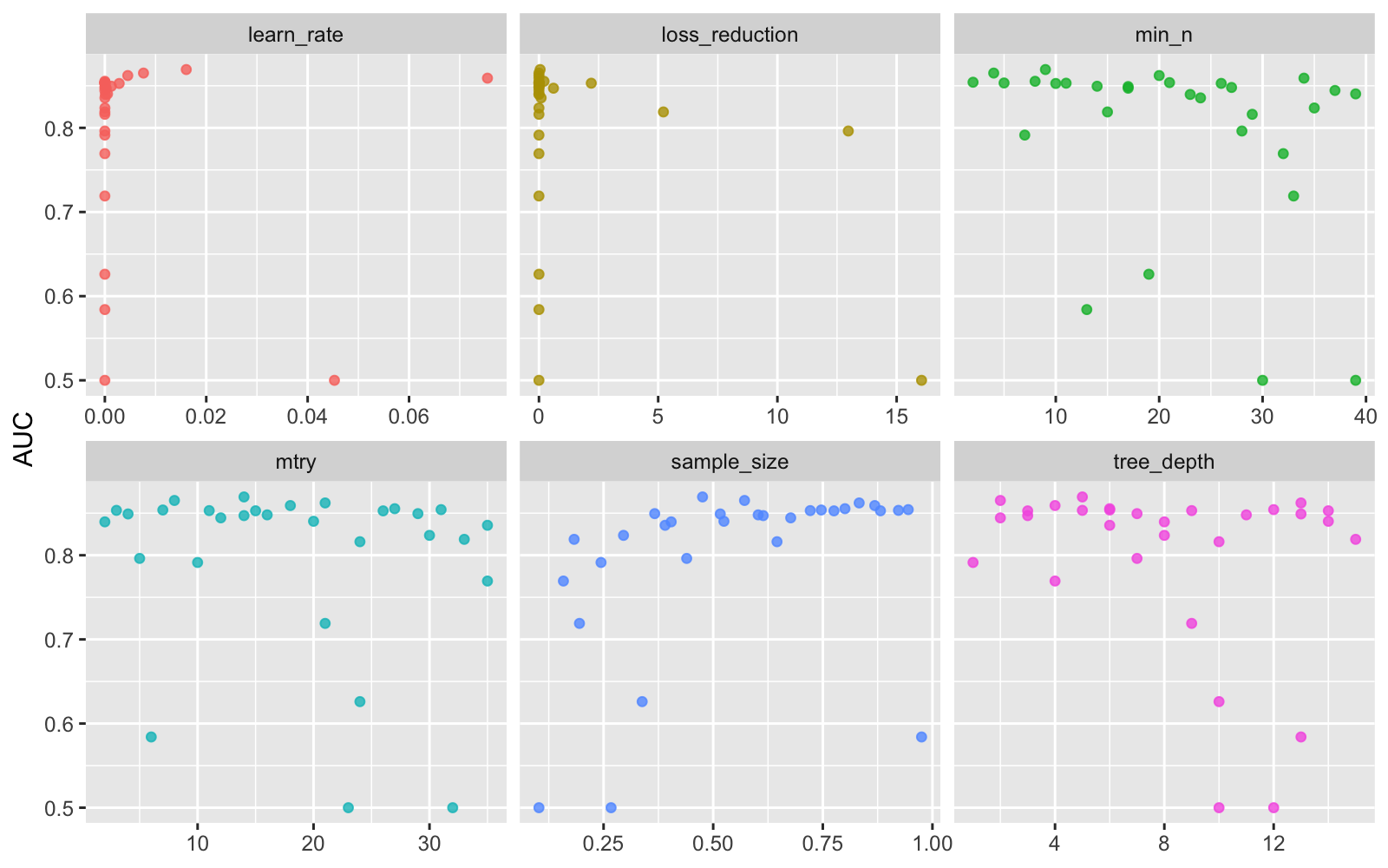

show_best(xgb_res, "roc_auc")

## # A tibble: 5 x 11
##    mtry min_n tree_depth learn_rate loss_reduction sample_size .metric
##   <int> <int>      <int>      <dbl>          <dbl>       <dbl> <chr>  
## 1    14     9          5 0.0161     0.0498               0.476 roc_auc
## 2     8     4          2 0.00762    0.000000158          0.571 roc_auc
## 3    21    20         13 0.00452    0.000000000144       0.833 roc_auc
## 4    18    34          4 0.0755     0.00000593           0.868 roc_auc
## 5    27     8          6 0.00000177 0.214                0.801 roc_auc
## # … with 4 more variables: .estimator <chr>, mean <dbl>, n <int>, std_err <dbl>

best_auc <- select_best(xgb_res, "roc_auc")
best_auc

## # A tibble: 1 x 6
##    mtry min_n tree_depth learn_rate loss_reduction sample_size
##   <int> <int>      <int>      <dbl>          <dbl>       <dbl>
## 1    14     9          5     0.0161         0.0498       0.476

Yet another set of tune functions to check what are the best performing sets of parameters and selecting the best

final_xgb <- finalize_workflow(
  xgb_wf,
  best_auc)
final_xgb

## ══ Workflow ═══════════════════════════════════════════════════
## Preprocessor: Formula
## Model: boost_tree()
## 
## ── Preprocessor ───────────────────────────────────────────────
## is_regulatory ~ .
## 
## ── Model ──────────────────────────────────────────────────────
## Boosted Tree Model Specification (classification)
## 
## Main Arguments:
##   mtry = 14
##   trees = 500
##   min_n = 9
##   tree_depth = 5
##   learn_rate = 0.0160598782732412
##   loss_reduction = 0.0498089052607873
##   sample_size = 0.475688168541528
## 
## Computational engine: xgboost

Finalizing the tuneable workflow with the best parameter

final_xgb %>%
  fit(data = feat_train) %>%
  pull_workflow_fit() %>%
  vip(geom = "point")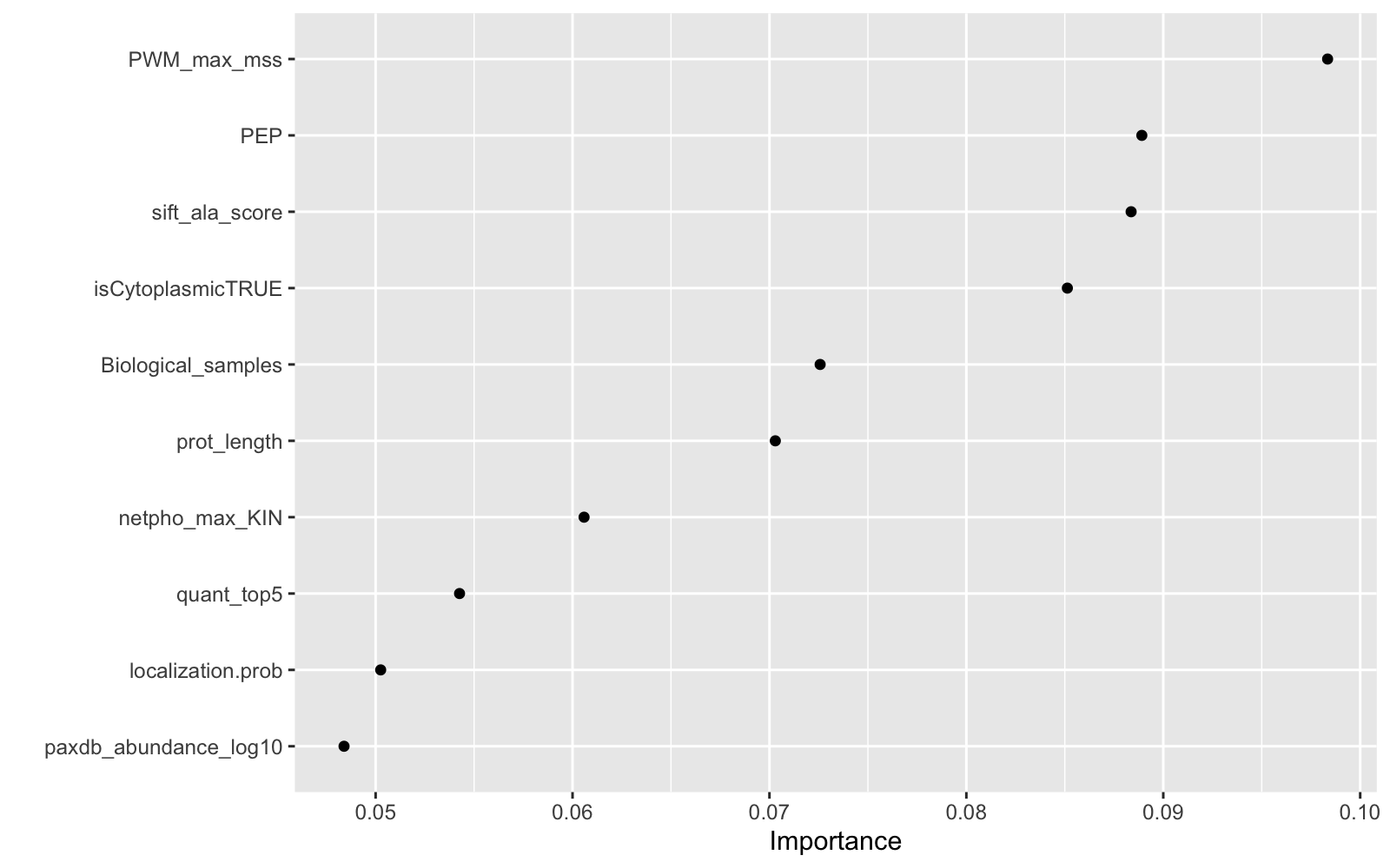

Showing what paremeters contribute most

Conclusions

As it was shown in Ochoa paper, the most informative feature for Tyrosine phosphorylation function is the Position Weight Matrices, PEP and number of different cell lines or tissues in which the site had been identified. This makes sense, since Phosphosite feeds from phosphoproteomics data.