Image Classification with CNN

Aug 21, 2020

Maria Dermit

16 minute read

Image Classification With Convolutional Neural Networks

In this article I will explore how to build a CNN using keras and classify images. My aim is to learn the basic of CNN, learn how use the tools to build them and use these tools to analyse digital pathology images.

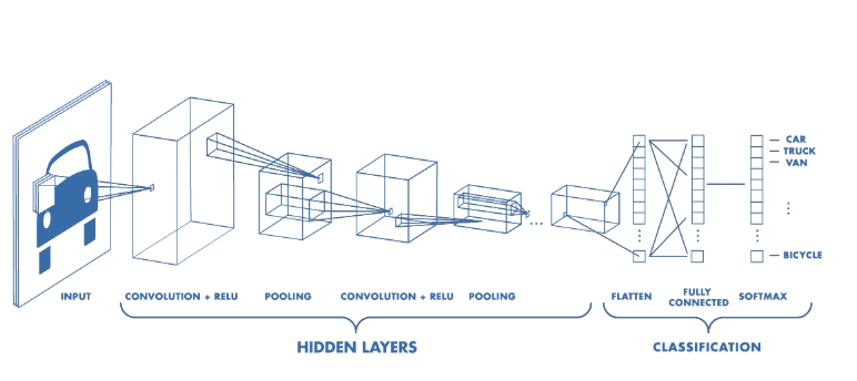
One popular way to do image classification is buy building Convolutional Neural Networks (CNN) using keras. CNN is a class of deep learning neural networks that uses a number of filters to extract features from images. In particular, CNN applies a series of convoluting (applying filter to modify the image) and pooling steps. In CNNs, sliding filters analyze pixels in groups with their neighbors and each filter can be dedicated to detecting a specific pattern in the image- so if the image is a face, there will be filters dedicated to detecting eyes, mouth or nose.

Filters start with random values and change along with the training process. So in the training these filters are getting trained to identifying unique features for each image type. In this process feature maps are generated and each filter triggers an activation function that determines whether a feature is present at each scanning position. This process goes throughout the layers of the CNN.

CNN

The state of the art in deep learning is provided by Keras and TensorFlow (if you are interested in learning more about some of their key features you can visit. In addition to image classification, Keras canbe used for text-classification too.

In this example of image classification I am going to use a model to classify a small number (7) of images from:

Standard Bikes.
Electric Bikes.
Scooters.

I decided to use these type of images because my human eye would have a pretty hard time telling apart Standard Bikes from Electric Bikes. The main different feature between these types of bikes is that Electric Bikes have a big bock on the frame or at the bike fork. I got jpg images from Google and the file size is different for all of them. Also, some of them have different backgrounds, so it is going to be interesting how the model handles that.

library(tidyverse)
library(here)
library(EBImage) #to read images 
library(keras) #to build the CNN model 
library(kableExtra) #to display tables

Getting the data

I can import the downloaded images using the function readImage from the EBImage package.

pics <- c(here("static","driving","b1.jpg"), here("static","driving","b2.jpg"),
          here("static","driving","b3.jpg"), here("static","driving","b4.jpg"),
          here("static","driving","b5.jpg"), here("static","driving","b6.jpg"),
          here("static","driving","b7.jpg"),
          here("static","driving","eb1.jpg"),here("static","driving","eb2.jpg"),
          here("static","driving","eb3.jpg"),here("static","driving","eb4.jpg"),
          here("static","driving","eb5.jpg"),here("static","driving","eb6.jpg"),
          here("static","driving","eb7.jpg"),
          here("static","driving","s1.jpg"), here("static","driving","s2.jpg"),
          here("static","driving","s3.jpg"), here("static","driving","s4.jpg"),
          here("static","driving","s5.jpg"), here("static","driving","s6.jpg"),
          here("static","driving","s7.jpg"))
mypic <- list()
for (i in 1:length(pics)) {mypic[[i]] <- readImage(pics[i])}

Exploring the data

print(mypic[[1]])

## Image 
##   colorMode    : Color 
##   storage.mode : double 
##   dim          : 1000 725 3 
##   frames.total : 3 
##   frames.render: 1 
## 
## imageData(object)[1:5,1:6,1]
##      [,1] [,2] [,3] [,4] [,5] [,6]
## [1,]    1    1    1    1    1    1
## [2,]    1    1    1    1    1    1
## [3,]    1    1    1    1    1    1
## [4,]    1    1    1    1    1    1
## [5,]    1    1    1    1    1    1

display(mypic[[8]])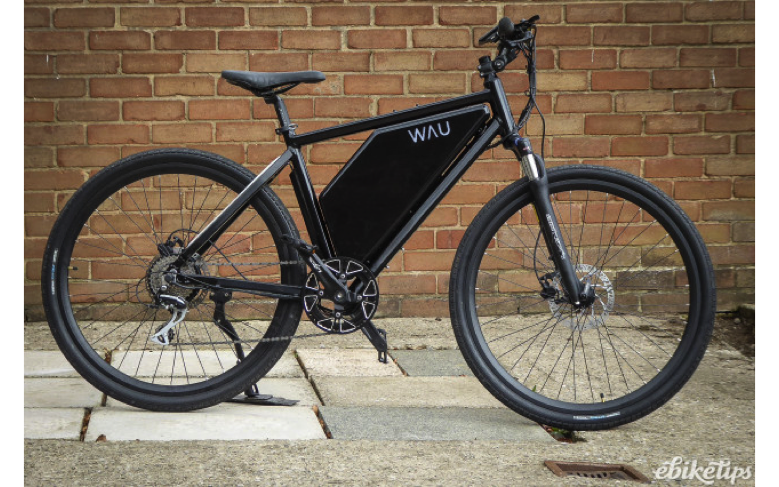

summary(mypic[[1]])

##    Min. 1st Qu.  Median    Mean 3rd Qu.    Max. 
##  0.0000  0.7412  1.0000  0.8169  1.0000  1.0000

hist(mypic[[2]])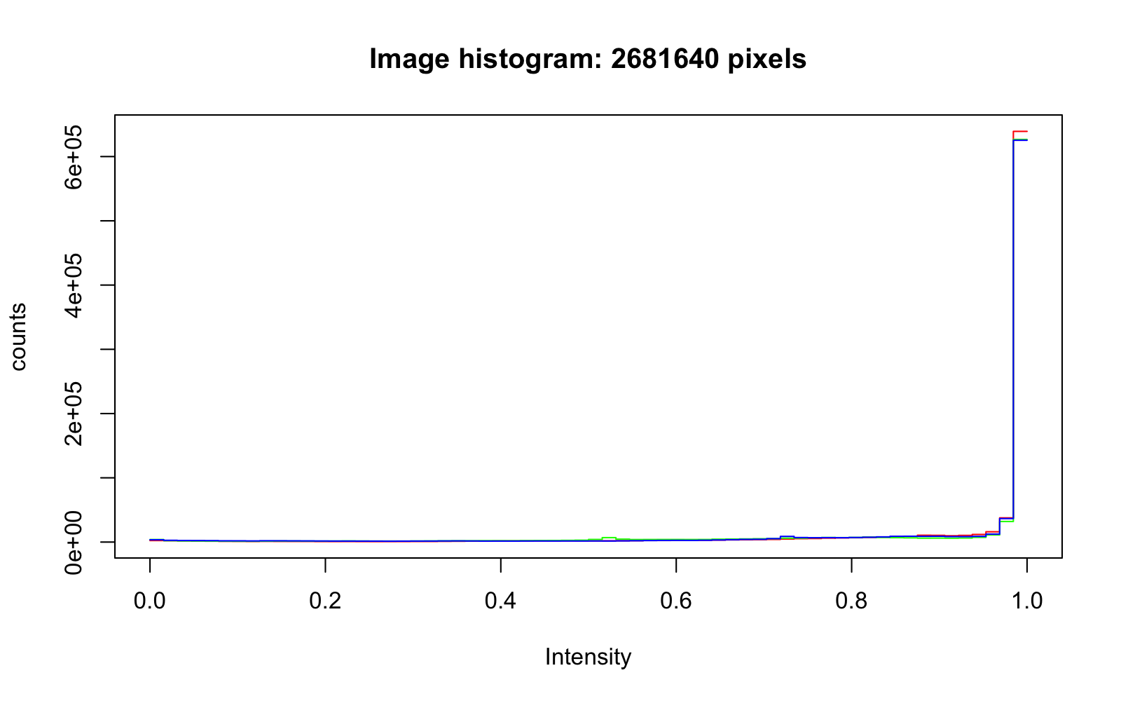

str(mypic)

## List of 21
##  $ :Formal class 'Image' [package "EBImage"] with 2 slots
##   .. ..@ .Data    : num [1:1000, 1:725, 1:3] 1 1 1 1 1 1 1 1 1 1 ...
##   .. ..@ colormode: int 2
##  $ :Formal class 'Image' [package "EBImage"] with 2 slots
##   .. ..@ .Data    : num [1:1170, 1:764, 1:3] 1 1 1 1 1 1 1 1 1 1 ...
##   .. ..@ colormode: int 2
##  $ :Formal class 'Image' [package "EBImage"] with 2 slots
##   .. ..@ .Data    : num [1:880, 1:530, 1:3] 1 1 1 1 1 1 1 1 1 1 ...
##   .. ..@ colormode: int 2
##  $ :Formal class 'Image' [package "EBImage"] with 2 slots
##   .. ..@ .Data    : num [1:1000, 1:660, 1:3] 1 1 1 1 1 1 1 1 1 1 ...
##   .. ..@ colormode: int 2
##  $ :Formal class 'Image' [package "EBImage"] with 2 slots
##   .. ..@ .Data    : num [1:500, 1:333, 1:3] 0.173 0.176 0.176 0.169 0.173 ...
##   .. ..@ colormode: int 2
##  $ :Formal class 'Image' [package "EBImage"] with 2 slots
##   .. ..@ .Data    : num [1:2000, 1:1284, 1:3] 1 1 1 1 1 1 1 1 1 1 ...
##   .. ..@ colormode: int 2
##  $ :Formal class 'Image' [package "EBImage"] with 2 slots
##   .. ..@ .Data    : num [1:286, 1:176, 1:3] 1 1 1 1 1 1 1 1 1 1 ...
##   .. ..@ colormode: int 2
##  $ :Formal class 'Image' [package "EBImage"] with 2 slots
##   .. ..@ .Data    : num [1:640, 1:426, 1:3] 0.4 0.447 0.467 0.455 0.471 ...
##   .. ..@ colormode: int 2
##  $ :Formal class 'Image' [package "EBImage"] with 2 slots
##   .. ..@ .Data    : num [1:4740, 1:2916, 1:3] 1 1 1 1 1 1 1 1 1 1 ...
##   .. ..@ colormode: int 2
##  $ :Formal class 'Image' [package "EBImage"] with 2 slots
##   .. ..@ .Data    : num [1:1500, 1:1272, 1:3] 1 1 1 1 1 1 1 1 1 1 ...
##   .. ..@ colormode: int 2
##  $ :Formal class 'Image' [package "EBImage"] with 2 slots
##   .. ..@ .Data    : num [1:800, 1:458, 1:3] 1 1 1 1 1 1 1 1 1 1 ...
##   .. ..@ colormode: int 2
##  $ :Formal class 'Image' [package "EBImage"] with 2 slots
##   .. ..@ .Data    : num [1:1200, 1:900, 1:3] 0.322 0.306 0.325 0.349 0.353 ...
##   .. ..@ colormode: int 2
##  $ :Formal class 'Image' [package "EBImage"] with 2 slots
##   .. ..@ .Data    : num [1:1620, 1:1080, 1:3] 1 1 1 1 1 1 1 1 1 1 ...
##   .. ..@ colormode: int 2
##  $ :Formal class 'Image' [package "EBImage"] with 2 slots
##   .. ..@ .Data    : num [1:1000, 1:667, 1:3] 1 1 1 1 1 1 1 1 1 1 ...
##   .. ..@ colormode: int 2
##  $ :Formal class 'Image' [package "EBImage"] with 2 slots
##   .. ..@ .Data    : num [1:2000, 1:2000, 1:3] 1 1 1 1 1 1 1 1 1 1 ...
##   .. ..@ colormode: int 2
##  $ :Formal class 'Image' [package "EBImage"] with 2 slots
##   .. ..@ .Data    : num [1:306, 1:512, 1:3] 1 1 1 1 1 1 1 1 1 1 ...
##   .. ..@ colormode: int 2
##  $ :Formal class 'Image' [package "EBImage"] with 2 slots
##   .. ..@ .Data    : num [1:670, 1:544, 1:3] 1 1 1 1 1 1 1 1 1 1 ...
##   .. ..@ colormode: int 2
##  $ :Formal class 'Image' [package "EBImage"] with 2 slots
##   .. ..@ .Data    : num [1:800, 1:800, 1:3] 1 1 1 1 1 1 1 1 1 1 ...
##   .. ..@ colormode: int 2
##  $ :Formal class 'Image' [package "EBImage"] with 2 slots
##   .. ..@ .Data    : num [1:1000, 1:1000, 1:3] 1 1 1 1 1 1 1 1 1 1 ...
##   .. ..@ colormode: int 2
##  $ :Formal class 'Image' [package "EBImage"] with 2 slots
##   .. ..@ .Data    : num [1:843, 1:640, 1:3] 1 1 1 1 1 1 1 1 1 1 ...
##   .. ..@ colormode: int 2
##  $ :Formal class 'Image' [package "EBImage"] with 2 slots
##   .. ..@ .Data    : num [1:900, 1:900, 1:3] 0.969 0.969 0.969 0.969 0.969 ...
##   .. ..@ colormode: int 2

Splitting for train/testing

This will ensure that our data has a split between 70/30 and 80/20 training/testing which is standard for training CNN model. So from the 7 set of each image class we take 5 images for training and 2 images for testing.

trainX <- list(1:16)

for(x in 1:5){
  trainX[[x]] <- mypic[[x]] #bikes
  trainX[[x+5]] <- mypic[[x+7]] #ebikes
  trainX[[x+10]] <-mypic[[x+14]] #scooters
}

testX <- list(1:6)

#select last two images in each group
for(x in 1:2){
  testX[[x]] <- mypic[[x+5]] #bikes
  testX[[x+2]] <- mypic[[x+12]] #ebikes
  testX[[x+4]] <- mypic[[x+19]] #scooters
}

Preparing the data

To prepare the data for training and testing we want to keep all image dimensions constant; as I sayed I downloaded images from Google and they came in different sizes. We need to resize the images so that all are 176 by 176 pixels using resize function from the EBImage Library. I chose 176 by 176 because it was smaller than the smallest height across all the the dataset. Images must also have equal width and height (square dimensions) because we want to end up with square matrices.

#Resizing Images (Train)
for(x in 1:length(trainX)){
  trainX[[x]] <- resize(trainX[[x]], 176, 176)
}

#Resizing Images (test)
for(x in 1:length(testX)){
  testX[[x]] <- resize(testX[[x]], 176, 176)
}

#Display new dimensions
#str(trainX)
str(testX)

## List of 6
##  $ :Formal class 'Image' [package "EBImage"] with 2 slots
##   .. ..@ .Data    : num [1:176, 1:176, 1:3] 1 1 1 1 1 1 1 1 1 1 ...
##   .. ..@ colormode: int 2
##  $ :Formal class 'Image' [package "EBImage"] with 2 slots
##   .. ..@ .Data    : num [1:176, 1:176, 1:3] 1 1 1 1 1 1 1 1 1 1 ...
##   .. ..@ colormode: int 2
##  $ :Formal class 'Image' [package "EBImage"] with 2 slots
##   .. ..@ .Data    : num [1:176, 1:176, 1:3] 1 1 1 1 1 1 1 1 1 1 ...
##   .. ..@ colormode: int 2
##  $ :Formal class 'Image' [package "EBImage"] with 2 slots
##   .. ..@ .Data    : num [1:176, 1:176, 1:3] 1 1 1 1 1 1 1 1 1 1 ...
##   .. ..@ colormode: int 2
##  $ :Formal class 'Image' [package "EBImage"] with 2 slots
##   .. ..@ .Data    : num [1:176, 1:176, 1:3] 1 1 1 1 1 1 1 1 1 1 ...
##   .. ..@ colormode: int 2
##  $ :Formal class 'Image' [package "EBImage"] with 2 slots
##   .. ..@ .Data    : num [1:176, 1:176, 1:3] 0.969 0.969 0.969 0.969 0.969 ...
##   .. ..@ colormode: int 2

Combining the data together and

We can use combine to merge all separated images into an image sequence and display them using display, both functions from EBImage.

trainX <- combine(trainX)
dis <- tile(trainX, 5)
display(dis, title = "Eco mobility")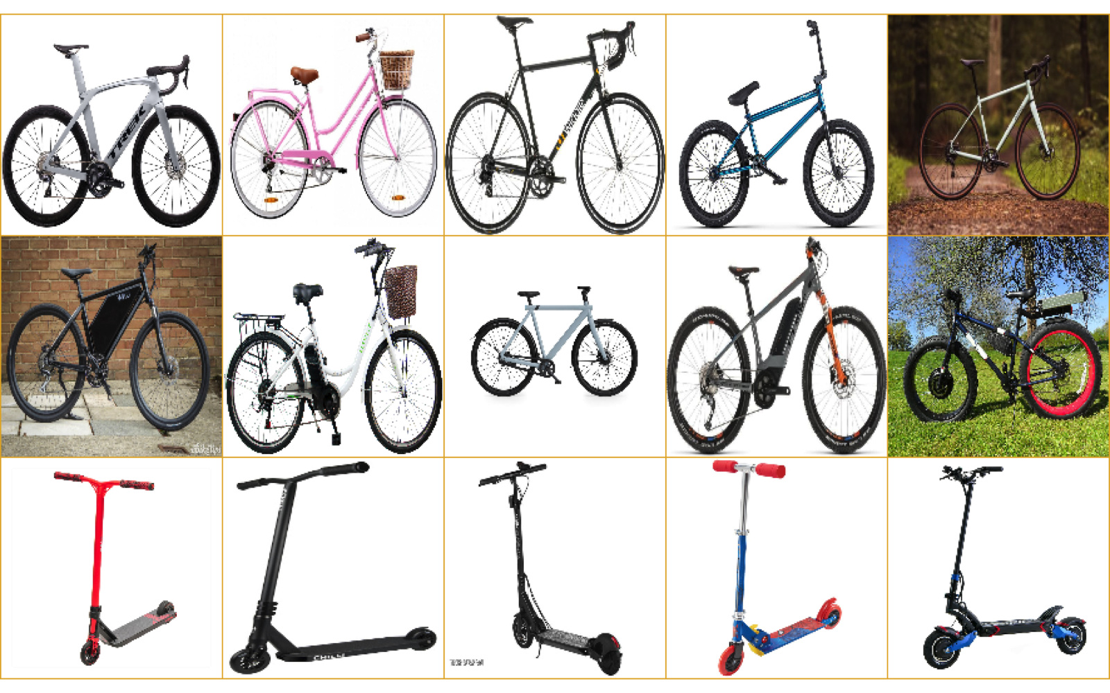

We can see that most pictures have a white background, but some of them have a background with a park or a wall.

testX <- combine(testX)
dis2 <- tile(testX, 2)
display(dis2, title = "Eco mobility")

str(testX)

## Formal class 'Image' [package "EBImage"] with 2 slots
##   ..@ .Data    : num [1:176, 1:176, 1:3, 1:6] 1 1 1 1 1 1 1 1 1 1 ...
##   ..@ colormode: int 2

We need to reorder the dimensions (number of images, width, height, color), and we can use the aperm to do this permutation.

testX <- aperm(testX, c(4,1,2,3))
trainX <- aperm(trainX, c(4, 1, 2, 3))

str(testX)

##  num [1:6, 1:176, 1:176, 1:3] 1 1 1 1 1 ...

Creating labels

We are going to give labels to each category, so: - Standard Bikes get 0 - Electric Bikes get 1 - Scooters get 2

trainY <- c(rep(0, 5), rep(1, 5), rep(2,5))
testY <- c(0,0,1,1,2,2)

One Hot Encoding

We now have the data splitted, resized andwe have created labels. The next step we need to do is One Hot Encoding, which basically transform the vector that contains the values for each class to a matrix with a boolean value for each class.

We can use the to_categorical function to do this.

#One Hot Encoding
trainLabels <- to_categorical(trainY)
testLabels <- to_categorical(testY)

#Display matrix
kable(testLabels) %>%
  kable_styling() %>%
  scroll_box(width = "100%", height = "200px")

1	0	0
1	0	0
0	1	0
0	1	0
0	0	1
0	0	1

Building the model

Building the neural network requires configuring the layers of the model and then compiling the model. Layers are the building block of a neural network, and they extract representations from the data fed into them. To create a sequential model we can use the keras_model_sequential function and then add series of layer functions. Adding layers reminds me of adding steps in tidymodels.

Our model has to differentiate if an image is a bike, an ebike or a scooter, and this is reflected by binary 1 and 0 values. A type of network that performs well on such a problem is a multi-layer perceptron. This type of neural network has classifiers that are fully connected.There other type of layers, including convolution layers and pooling layes. As for activation function, a standard type is Rectified Linear Unit (RELU). Another activation function is softmax, which is used in the output layer, so that the output values are between 0 and 1, which make it easy to work with predicted probabilities.

Once the model gets build, we need to compile it, and to do so we can call categorical_crossentropy loss function and use a particular optimiser algorithm, like Stochastic Gradient Descent (sgd). Finally, to monitor the model accuracy during we can use metrics accuracy.

model <- keras_model_sequential()
model %>%
  layer_conv_2d(filters = 32, kernel_size = c(3,3), activation = 'relu',   input_shape = c(176, 176, 3)) %>%
  layer_conv_2d(filters = 32, kernel_size = c(3,3) , activation = 'relu') %>%
  layer_max_pooling_2d(pool_size = c(2,2)) %>%
  layer_dropout(rate = 0.25) %>%
  layer_conv_2d(filters = 64, kernel_size = c(3,3), activation = 'relu')%>%
  layer_conv_2d(filters = 64, kernel_size = c(3,3), activation = 'relu') %>%
  layer_max_pooling_2d(pool_size = c(2,2)) %>%
  layer_dropout(rate = 0.25) %>%
  layer_flatten() %>% #this allows to pass to next layer, which is always dense
  layer_dense(units = 256, activation = 'relu') %>%
  layer_dropout(rate = 0.25) %>%
  layer_dense(units = 3, activation = "softmax") %>%
  compile(loss = "categorical_crossentropy", 
          optimizer = 
            optimizer_sgd(lr = 0.001, momentum = 0.9, decay = 1e-6, nesterov = T),
          metrics = c('accuracy'))
  
#View the model
summary(model)

## Model: "sequential"
## ________________________________________________________________________________
## Layer (type)                        Output Shape                    Param #     
## ================================================================================
## conv2d (Conv2D)                     (None, 174, 174, 32)            896         
## ________________________________________________________________________________
## conv2d_1 (Conv2D)                   (None, 172, 172, 32)            9248        
## ________________________________________________________________________________
## max_pooling2d (MaxPooling2D)        (None, 86, 86, 32)              0           
## ________________________________________________________________________________
## dropout (Dropout)                   (None, 86, 86, 32)              0           
## ________________________________________________________________________________
## conv2d_2 (Conv2D)                   (None, 84, 84, 64)              18496       
## ________________________________________________________________________________
## conv2d_3 (Conv2D)                   (None, 82, 82, 64)              36928       
## ________________________________________________________________________________
## max_pooling2d_1 (MaxPooling2D)      (None, 41, 41, 64)              0           
## ________________________________________________________________________________
## dropout_1 (Dropout)                 (None, 41, 41, 64)              0           
## ________________________________________________________________________________
## flatten (Flatten)                   (None, 107584)                  0           
## ________________________________________________________________________________
## dense (Dense)                       (None, 256)                     27541760    
## ________________________________________________________________________________
## dropout_2 (Dropout)                 (None, 256)                     0           
## ________________________________________________________________________________
## dense_1 (Dense)                     (None, 3)                       771         
## ================================================================================
## Total params: 27,608,099
## Trainable params: 27,608,099
## Non-trainable params: 0
## ________________________________________________________________________________

Fitting the model

Now that we have built the architecture of the model and the image data is processed, we are ready to integrate the two. To do this we use the fit function from keras with the training data and traning labels. Some hyperparameters that are defined are:

history <- model %>%
  fit(trainX, trainLabels, 
      epochs = 60, #times the training set gets passed through the CNN for optimization
      batch_size = 32,#samples propagated through the CNN at one time 
      validation_split = 0.2 #percent of training data used for validation
      )

#Visualising the fitting/ epochs
plot(history)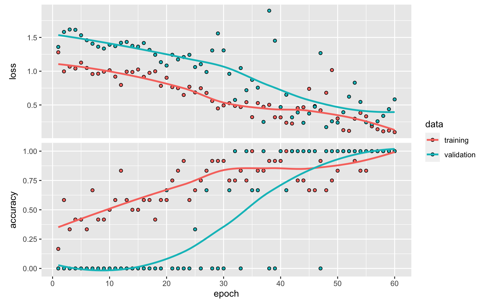

loss and acc indicate the loss and accuracy of the model for the training data.
val_loss and val_acc aindicate the loss and accuracy of the model for the for the test or validation data.

We can see that with each iteration the loss decreasing and the accuracy increasing. But are we overfitting? Has the model over-learnt the training dataset?

There may be some sings of overfitting if the training data accuracy keeps improving while the validation data accuracy gets worse (model starts to just memorize the data instead of learning from it). A solution when this happens can be doing data augmentation. On the other hand, if the trend for accuracy on both datasets is still rising for the last few epochs, this may be a sign that the model has not yet over-learned the training dataset.

We have now trained the model, compiled it and fitted to data so we can adjust hyperparameters and other factors to optimize the accuracy.

Evaluating the model

On the train data.

evTrain <- model %>%
  evaluate(trainX, trainLabels)
evTrain

##      loss  accuracy 
## 0.2641464 1.0000000

This model had a 100% accuracy for predicting the training set with loss of 16.86%.

We can call predict_classes to use the model to make a prediction of the training set and create a confusion matrix.

pred <- model %>%
  predict_classes(trainX)

#Create the confusion matrix
table(Predicted = pred, Actual = trainY)

##          Actual
## Predicted 0 1 2
##         0 5 0 0
##         1 0 5 0
##         2 0 0 5

The confusion matrix shows that the model we created makes the right predictions.

We can look at the probabilities for each categories.

prob <- model %>%
  predict_proba(trainX)

cbind(prob, Predicted_class = pred, Actual = trainY)

##                                        Predicted_class Actual
##  [1,] 0.95703465 0.03201567 0.01094964               0      0
##  [2,] 0.86703885 0.06097450 0.07198658               0      0
##  [3,] 0.93079931 0.04088598 0.02831475               0      0
##  [4,] 0.96321779 0.02021343 0.01656874               0      0
##  [5,] 0.81137061 0.14501296 0.04361647               0      0
##  [6,] 0.16804671 0.78936154 0.04259172               1      1
##  [7,] 0.19521724 0.76894486 0.03583783               1      1
##  [8,] 0.25084555 0.59466624 0.15448825               1      1
##  [9,] 0.11676817 0.86339182 0.01983995               1      1
## [10,] 0.22755799 0.68718290 0.08525907               1      1
## [11,] 0.08194190 0.03500600 0.88305211               2      2
## [12,] 0.03219539 0.01162616 0.95617843               2      2
## [13,] 0.42813191 0.08656579 0.48530233               2      2
## [14,] 0.33236235 0.06212686 0.60551077               2      2
## [15,] 0.33998162 0.06697037 0.59304798               2      2

It looks like the model does not have issues predicting images with bicycles correctly.This looks quite surprising, since the standard bikes and ebikes look so similar to me!

On the test data.

We can repeat the above steps for test data.

evTest <- model %>%
  evaluate(testX, testLabels)
evTest

##      loss  accuracy 
## 0.5950766 0.6666667

We can see than in the accuracy on the test data drops. This could be due to the fact that 5 images per group for test and train data set is way too small of a sample and also there was variations in images and backgrounds. Plus, accuracies fluctuate every time the model runs.

predTest <- model %>%
  predict_classes(testX)

#Create the confusion matrix
table(Predicted = predTest, Actual = testY)

##          Actual
## Predicted 0 1 2
##         0 2 2 0
##         2 0 0 2

In fact we can see that the model has some issues to distinguish standard bikes and ebikes when seeing new data. No issues to tell scooters apart.

probTest <- model %>%
  predict_proba(testX)
cbind(probTest, Predicted_class = predTest, Actual = testY)

##                                      Predicted_class Actual
## [1,] 0.9484544 0.03665487 0.01489069               0      0
## [2,] 0.9180664 0.05786508 0.02406845               0      0
## [3,] 0.4268365 0.34671259 0.22645089               0      1
## [4,] 0.5001020 0.21784234 0.28205565               0      1
## [5,] 0.1583756 0.03504702 0.80657738               2      2
## [6,] 0.3862076 0.08324913 0.53054321               2      2

ggplot() +
  geom_col(aes(x = c("Training", "Testing"), y = c(evTrain[2], evTest[2])), fill = c("green", "darkgreen")) +
  geom_text(aes(x = c("Training", "Testing"), y = c(evTrain[2] + 0.1 , evTest[2] + 0.1), label = c(round(evTrain[2], 2), round(evTest[2], 2)))) +
  labs(y = "Accuracy", x ="Data", title = "Accuracy of Train & Test Data ") +
   theme(plot.title = element_text(hjust = 0.5), legend.position = "top")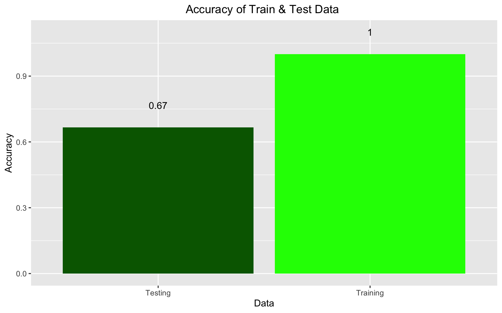

Conclusions

Keras provides an interphase to build and optimise CNN models
This model had very little number of images the our training and testing set. Adding more data to the model will push accuracy higher. This would also require a GPU (if not it might just take forever to run). One could leverage cloud computing with clouldml to train on GPUs.
Increasing the number of layers may help on decreasing loss.