Getting data

smile_raw<-genius_album(artist = "Katy Perry", album = "Smile")

Data preparation

tidy_smile <- smile_raw %>%
  unnest_tokens(word, lyric)

tidy_smile  %>% count(track_title)

## # A tibble: 12 x 2
##    track_title                  n
##    <chr>                    <int>
##  1 Champagne Problems          18
##  2 Cry About It Later          92
##  3 Daisies                      1
##  4 Harleys in Hawaii          339
##  5 Never Really Over            1
##  6 Not the End of the World    60
##  7 Only Love                   18
##  8 Resilient                  213
##  9 Smile                      333
## 10 Teary Eyes                  81
## 11 Tucked                       1
## 12 What Makes a Woman           1

smile_raw %>% filter(track_title=="Tucked")

## # A tibble: 1 x 4
##   track_n  line lyric track_title
##     <int> <int> <chr> <chr>      
## 1       9    NA <NA>  Tucked

We can do text analysis using the fantastic tidytext package. To use tidytext, we need to tokenise words to extract meaning and use tidytext’s sentiment analysis capabilities. We can use unnest_tokens function uses the tokenizers package to separate each lyric line into words. The default tokenizing is for words, but other options include characters, n-grams, sentences, lines, paragraphs, or separation around a regex pattern. We realised the lyrics of some songs have yet to be released.

tidy_smile <- tidy_smile %>%
  anti_join(get_stopwords())

We can remove stop words (available via the function get_stopwords()) with an anti_join(). Lets count the frequency of words.

tidy_smile %>%
  count(word, sort = TRUE) 

## # A tibble: 233 x 2
##    word         n
##    <chr>    <int>
##  1 smile       19
##  2 oh          17
##  3 baby        16
##  4 back        15
##  5 now         15
##  6 cause       13
##  7 finally     12
##  8 got         11
##  9 grateful    11
## 10 jeweler     11
## # … with 223 more rows

There is a range of methods and dictionaries for evaluating the opinion or emotion in text. The tidytext package comes with several sentiment lexicons.

get_sentiments("bing") %>% count(sentiment)

## # A tibble: 2 x 2
##   sentiment     n
##   <chr>     <int>
## 1 negative   4781
## 2 positive   2005

get_sentiments("nrc") %>% count(sentiment)

## # A tibble: 10 x 2
##    sentiment        n
##    <chr>        <int>
##  1 anger         1247
##  2 anticipation   839
##  3 disgust       1058
##  4 fear          1476
##  5 joy            689
##  6 negative      3324
##  7 positive      2312
##  8 sadness       1191
##  9 surprise       534
## 10 trust         1231

get_sentiments("loughran") %>% count(sentiment)

## # A tibble: 6 x 2
##   sentiment        n
##   <chr>        <int>
## 1 constraining   184
## 2 litigious      904
## 3 negative      2355
## 4 positive       354
## 5 superfluous     56
## 6 uncertainty    297

Sentiment analysis

In this analysis I am going to use 2 lexicons:

• bing by Liu and collaborators

• nrc by Saif Mohammad and Peter Turney.

smile_sentiment <- tidy_smile %>%
  inner_join(get_sentiments("bing"), by = "word") %>% 
  count(track_title, sentiment) %>% 
  spread(sentiment, n, fill = 0) %>% 
  mutate(sentiment = positive - negative)
smile_sentiment

## # A tibble: 6 x 4
##   track_title              negative positive sentiment
##   <chr>                       <dbl>    <dbl>     <dbl>
## 1 Cry About It Later              5        6         1
## 2 Harleys in Hawaii               0        4         4
## 3 Not the End of the World        4        2        -2
## 4 Resilient                       6       15         9
## 5 Smile                          13       56        43
## 6 Teary Eyes                      0        4         4

smile_sentiment_nrc <- tidy_smile %>%
  inner_join(get_sentiments("nrc"), by = "word") %>% 
  count(track_title, sentiment) 
smile_sentiment_nrc

## # A tibble: 50 x 3
##    track_title        sentiment        n
##    <chr>              <chr>        <int>
##  1 Cry About It Later anticipation     5
##  2 Cry About It Later joy              4
##  3 Cry About It Later negative         8
##  4 Cry About It Later positive         5
##  5 Cry About It Later sadness          4
##  6 Cry About It Later surprise         1
##  7 Cry About It Later trust            1
##  8 Harleys in Hawaii  anger            1
##  9 Harleys in Hawaii  anticipation     4
## 10 Harleys in Hawaii  disgust          1
## # … with 40 more rows

Plotting the data

ggplot(smile_sentiment, aes(track_title, sentiment, fill = track_title)) +
  geom_bar(stat = "identity", show.legend = FALSE)+
   theme_minimal(base_family = "")+
  theme(plot.title.position = "plot")+
  labs(x = "",
         y = "Sentiment",
         title = "Sentiment analysis per words across songs",
         subtitle = "Katty Perry's last album Smile")

BJTL

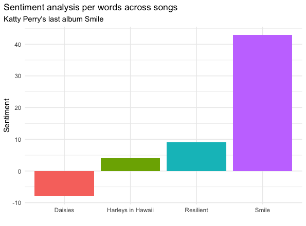
Despite the song called Daisies could sound bucolic, the song titled with this name has lowest sentiment rating (a.k.a more negative-associated words than positive-associated words).

ggplot(smile_sentiment_nrc, aes( n,sentiment, fill = track_title)) +
  geom_bar(stat = "identity", show.legend = FALSE)+
  theme_minimal(base_family = "")+
  theme(plot.title.position = "plot")+
  facet_wrap(~track_title, ncol = 2, scales="free") +
  labs(x = "",
         y = "Sentiment",title = "Sentiment analysis per words across songs",
         subtitle = "Katty Perry's last album Smile")

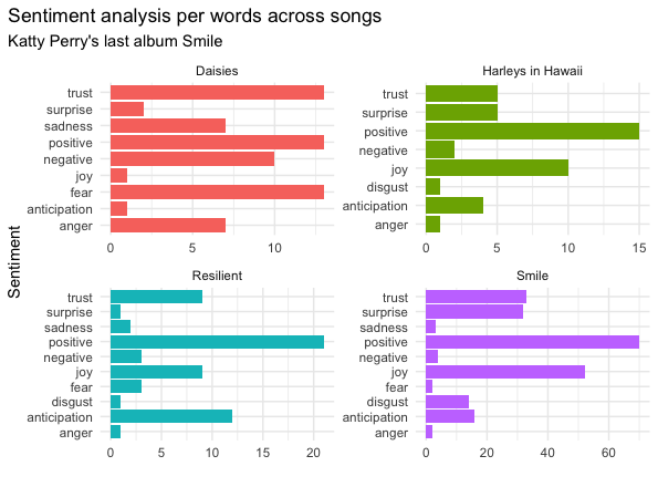
Overall, the songs have quite positive feelings/sentiments. Smile song has many positive and joyful terms and little fear-associated words. On the other hand, Daisies song, is the saddest song of the album, having as much fear as positive associated words and little joy.

Therefore, if you want to listen to the latest, more positive Katty Perry, click on the video image to watch her last song Smile 😄!