
Spotify
library(dplyr)
library(spotifyr)
library(plotly)
library(ggplot2)
library(ggjoy)
library(ggpubr)
library(rstatix)
library(wesanderson)
library(GGally)
Motivation to do this comparison
It is always a joke in my lab that Martin listens to better music than what I do. I find this utterly non-sense! To demonstrate my point, I analyse two artist Martin and I really like: on my case Rosalia and on Martin’s case The bouncing Souls. I took this information from his lab Spotify playlist.
Steps to do these analyses
First I get my client ID from Spotify
In Spotify for Developers I get my client id
Sys.setenv(SPOTIFY_CLIENT_ID = id)
Sys.setenv(SPOTIFY_CLIENT_SECRET = secret)
access_token <- get_spotify_access_token()
Then I get features for both artists
# Maria Music:Rosalia
maria_playlist <- get_playlist_audio_features(playlist_uris = '37i9dQZF1DXbjiU2ByCldP')
maria_playlist$researcher <- paste("maria")

#Martin Music: bouncing souls
martin_playlist <- get_playlist_audio_features(playlist_uris = '37i9dQZF1DZ06evO1WZiOk')
martin_playlist$researcher <- paste("martin")

lab_music <- rbind(maria_playlist, martin_playlist)
Overview of interesting features for each researcher
lab_music %>%
select(researcher,loudness,danceability, track.popularity) %>%
ggpairs(mapping = aes(color=researcher))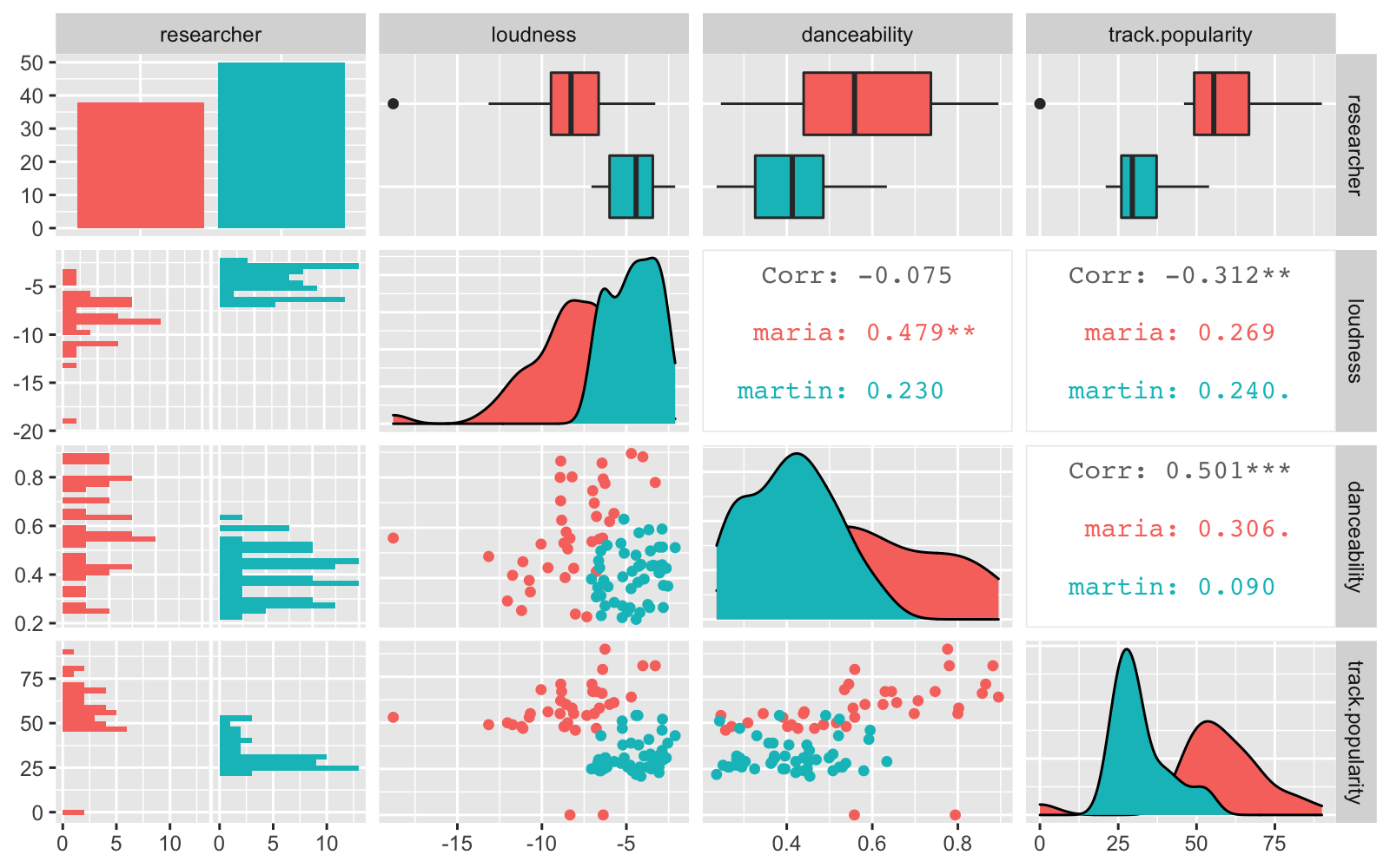 It looks like I listen to more popular and danceable music, and Martin’s music is louder than mine. According to Spotify, Danceability: describes how suitable a track is for dancing based on a combination of musical elements including tempo, rhythm stability, beat strength, and overall regularity. A value of 0.0 is least danceable and 1.0 is most danceable. This really comes at not surprise.
But the question is are the songs that I listen to is this difference in popularity significant?
How popular is the music Martin and I listen to?
p_value<-lab_music %>%
summarize(results = wilcox.test(track.popularity ~ researcher)$p.value)
stat.test <- lab_music %>%
wilcox_test(track.popularity ~ researcher, paired = FALSE)
lab_music %>%
mutate_if(is.character,as.factor) %>%
ggplot(aes(researcher,track.popularity, fill = researcher)) +
geom_boxplot() +
geom_point()+
xlab("") +
ylab("Popularity") +
geom_signif(annotations = stat.test$p,
y_position = 95, xmin=1, xmax=2) +
#stat_pvalue_manual(stat.test, x=researcher,label = "p") +
theme_classic()+
theme(plot.title.position = "plot",
plot.caption.position = "plot", legend.position = "none")+
labs(title = 'Popularity of song',
caption = "Maria-Rosalia\nMartin-The bouncing Souls")+
scale_fill_manual(values = wes_palette("Royal1"))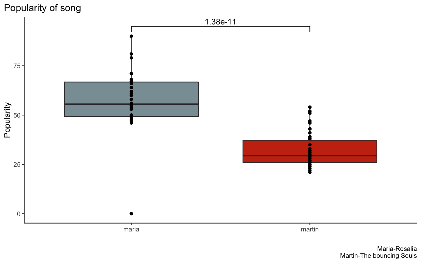 I listen to music that is more popular.
How danceable is the music Martin and I listen to?
p_value<-lab_music %>%
summarize(results = wilcox.test(danceability ~ researcher)$p.value)
stat.test <- lab_music %>%
wilcox_test(danceability ~ researcher, paired = FALSE)
lab_music %>%
mutate_if(is.character,as.factor) %>%
ggplot(aes(researcher,danceability, fill = researcher)) +
geom_boxplot() +
geom_point()+
xlab("") +
ylab("Danceability") +
geom_signif(annotations = stat.test$p,
y_position = 0.95, xmin=1, xmax=2) +
#stat_pvalue_manual(stat.test, x=researcher,label = "p") +
theme_classic()+
theme(plot.title.position = "plot",
plot.caption.position = "plot", legend.position = "none")+
labs(title = 'Danceability of song',
caption = "Maria-Rosalia\nMartin-The bouncing Souls")+
scale_fill_manual(values = wes_palette("Royal1"))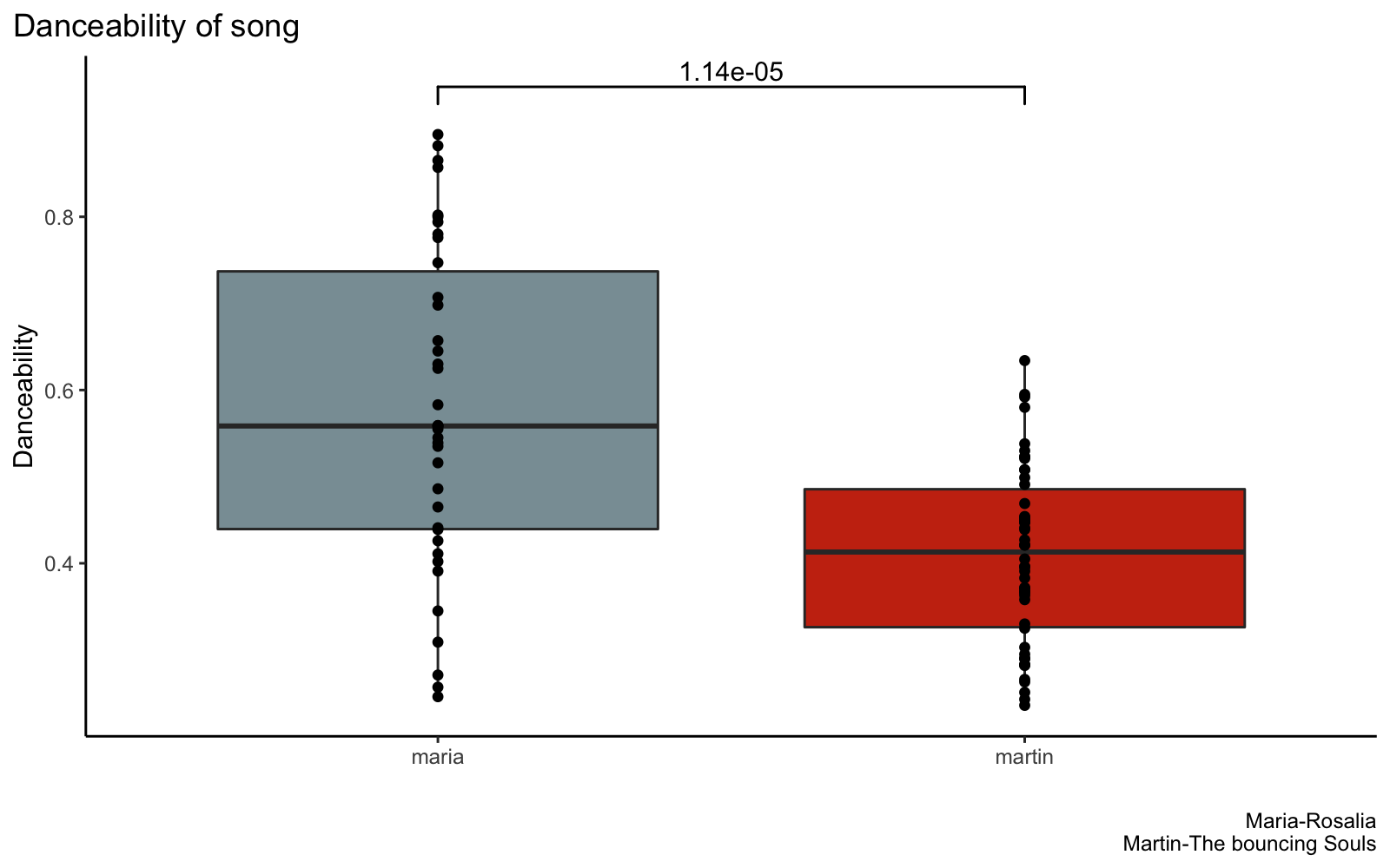 I listen to music that is more danceable.
How loud is the music Martin and I listen to?
p_value<-lab_music %>%
summarize(results = wilcox.test(loudness ~ researcher)$p.value)
stat.test <- lab_music %>%
wilcox_test(loudness ~ researcher, paired = FALSE)
lab_music %>%
mutate_if(is.character,as.factor) %>%
ggplot(aes(researcher,loudness, fill = researcher)) +
geom_boxplot() +
geom_point()+
xlab("") +
ylab("Loudness") +
geom_signif(annotations = stat.test$p,
y_position = 0.95, xmin=1, xmax=2) +
#stat_pvalue_manual(stat.test, x=researcher,label = "p") +
theme_classic()+
theme(plot.title.position = "plot",
plot.caption.position = "plot", legend.position = "none")+
labs(title = 'Loudness of song',
caption = "Maria-Rosalia\nMartin-The bouncing Souls")+
scale_fill_manual(values = wes_palette("Royal1"))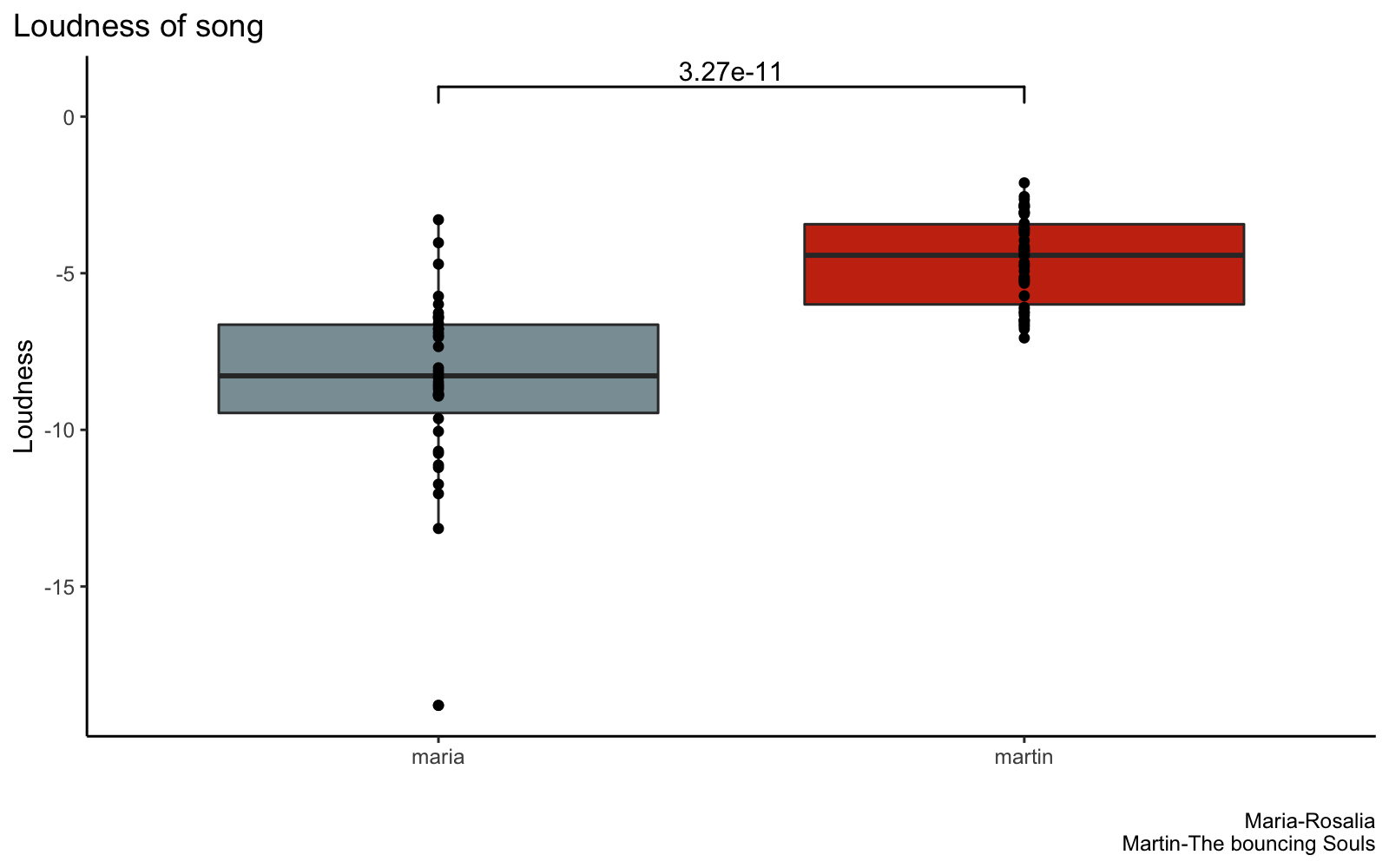 Interesting. Songs that Martin listens to are louder that the songs that I listen to. I found this tendency called Loudness war of music, the trend of increasing audio levels in recorded music, which reduces audio fidelity, and according to many critics, listener enjoyment. Has Martin fall into this trick and that is the reason he likes his music?


